The more data that appears on your spreadsheet, the more confusing it becomes. The filter function integrated in Microsoft Excel enables you to temporarily hide data that is not required and thus to have the relevant information in front of you at a glance. If you've already created an Excel spreadsheet, it already has a built-in filter. You can also either apply an AutoFilter to all columns or proceed individually. We will show you the options for filtering your content for both variants and how you can deactivate the filters again.
Text and number filters
Microsoft Excel offers you different filter options depending on the cell content. Whenever you click on the small arrow in the column heading, you will be shown a list of all values in the column. However, this makes less sense, especially for numerical values. Depending on whether there are text or number values in your column, number and text filters are suggested in the search field.
For example, if you click the small arrow > " Number filter "> " Greater than " for numerical values , you can set a lower limit for the displayed values.
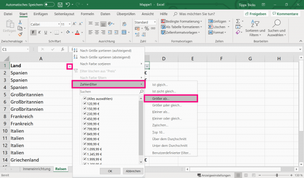
Note: Excel filters always hide the entire line as soon as the filter criterion has not been met..
AutoFilter
1st step:
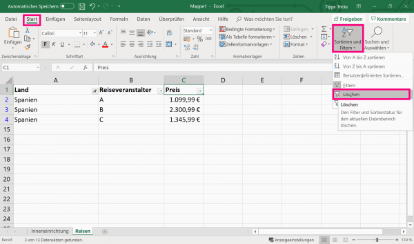
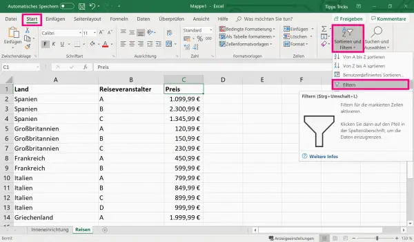 Go to " Sort and Filter " in the " Start " tab and then to " Filter ". If not all columns should be filtered, simply mark the column that you want to filter in advance.
2nd step:
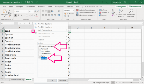 Arrow buttons are now automatically displayed in each column. With a click on the arrow you can select from a list in the expanded menu what you want to filter for. This process can be used for each column individually. However, you cannot create complex criteria with the help of the AutoFilter. There are special filters for this case .
Note: If you have already created data in Excel as a table, the column headings already have the AutoFilter. This is shown by the small arrow on the right-hand side of the heading. Select the arrow in the column where you want to create a filter. Click (Select All) in the list to clear all boxes. Now you can select the terms that should be filtered. Confirm your entry with " OK ".
Clear Filters
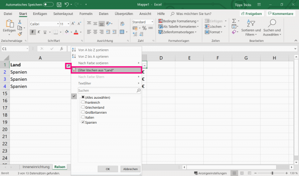
The filters created in Excel do not access your data directly. That means no matter which and how many filters you set, your data remains unchanged. If you want to remove filters completely, you can do this either for a single column or for all filters in the worksheet.
To delete the filter from a single column, click on the arrow button and then on " Delete filter from column title "..
If you would like to remove all filters in your worksheet, go to the " Data " tab and then click on " Filters " and then " Delete ".
Note: In addition to the filter functions, sorting functions (" From A to Z / From Z to A / Sort by color ") are also offered. Please note, however, that the re-sorting has a direct effect on the original data and cannot simply be deactivated - as with the filter function.
Special filters
Follow our step-by-step instructions or take a look at the brief instructions .
Brief instructions: special filters
- Above your data, leave 5 blank lines for the criteria area and label the columns. One line of this must remain free as a blank line.
- In the " Data " tab, click on " Filter ".
- Put in a new window List and Criteria range determined by the appropriate cells with the left mouse button Mark .
- You can then enter the criteria according to which the filter should be used in the criteria area. Use the following notation:
"="=Kriterium1" . You can use other comparison operators instead of the equal sign. - Now click again under " Data " and " Sort and Filter " on " Advanced " and choose between " List in the same place " if the lines for which the criteria do not apply should be hidden, or " To another place copy "if you want to paste the filtered data elsewhere in the worksheet.