Fix the first column 1st step 2nd step Freeze any column 1st step 2nd step 3rd step Remove the fixation Quick guide: Fix any column
With large tables, fixing rows and columns helps to maintain clarity. The fixed area of the worksheet remains visible, regardless of whether you scroll horizontally or vertically. You will never lose your bearings in extensive tables. If you want to change or remove the fixation, this is also done with just one click. We'll show you how it's done. After you've created a table in Excel, you can choose between several options.
Fix the first column
Follow our step-by-step instructions or take a look at the brief instructions .
1st step
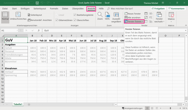 Switch to the " View " tab . Here you go to the point " Fix window ".
2nd step
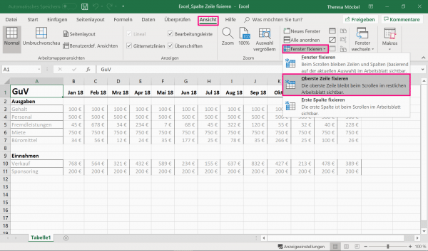 In the open drop-down menu, choose " first column fix ".
Freeze any column
Follow our step-by-step instructions or take a look at the brief instructions ..
Attention: Only consecutive rows and columns can be fixed.
1st step
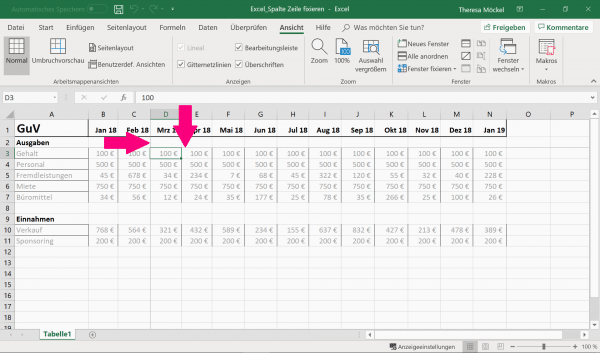
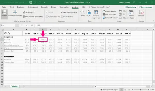 Select a cell . The fixation then takes effect for the column adjacent to the left and the line above (marked with arrows).
2nd step
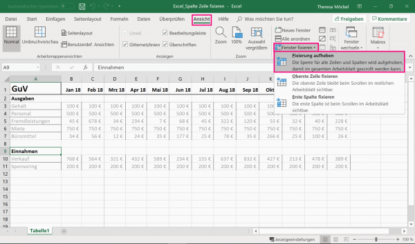
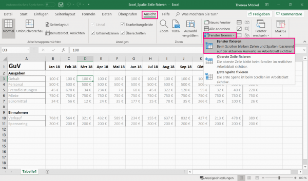 Now go to the " View " tab again on the symbol with the title " Fix window ". Here click again on " Freeze window ".
3rd step
 The fixation is indicated on your worksheet by a darker line color . You can scroll back and forth to check .
Remove the fixation
To unlock, you can be anywhere on the worksheet. Click on the " View " tab, then on " Freeze window " and then on " Unpin "..
Quick guide: Fix any column
1. Click in the cell from which the column on the left and the row above should be fixed.
2. In the " View " tab, go to " Freeze window ". Repeat entering " Freeze window " in the drop-down menu.
3. A darker line color highlights which area you have pinned. Scroll to test the fixation.