Use INDEX function 1st step: 2nd step: Combine INDEX with COMPARISON 1st step: 2nd step:
With the INDEX function of Excel you can read out a value based on the row and column position of a matrix. Sounds pretty simple actually. And that's it! To understand what the function does and how to use it correctly, read this guide.
You can also read tips about controls and formulas in Excel here.
Use INDEX function
1st step:
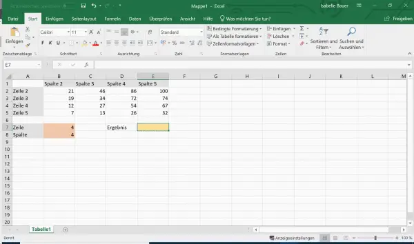 To search for a value in a matrix , you must first define your desired search parameters . In our example this is the value 4 for row and column. So we want to find out which value is in row 4, column 4.
2nd step:
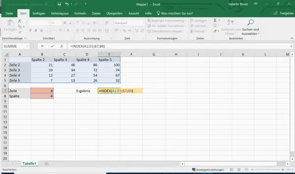 To use the INDEX function , first enter a search area . In our example this goes from A1 to E5. Then select the cells in which you previously entered the search parameters, i.e. B7 and B8. The function should look like this:
= INDEX (A1: E5, B7, B8)
The result in our example is the value 54, because this is in the cell where row 4 and column 4 cross.
Combine INDEX with COMPARISON
The INDEX function is rarely used alone. Because in order to look for a value, you have to know where it is within a range. And in a table with hundreds of entries, this is very tedious and time-consuming. Therefore INDEX is often used together with COMPARE..
1st step:
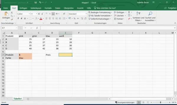 In our example, we would like to know how much product B in the color blue costs. So our search parameters are B and blue. Now enter the INDEX function again and define a search area (A1 to E5).
2nd step:
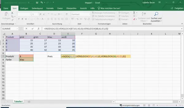 Instead of entering the search parameters now, expand the function with COMPARE . Now let Excel count the row or column in which the respective search parameter is located. Now select the cell with the search parameter again and then enter the search area for the respective parameter. In our example this is the range A1 to A5 for product B, and the range A1 to E1 for the color blue. At the end of the brackets, write a 0 , as there must be an exact match . The function should look like this:
= INDEX (A1: E5; COMPARE (B7; A1: A5; 0); COMPARE (B8; A1: E1; 0))
In our example, the result is the value 23, since this is located at the intersection of row 3 and column D.