Using the VLOOKUP formula in Excel is a breeze with the right tricks. The formula is used to find attributes in a list catalog. This can be easily explained using the example of a bookseller: Every book has a specific ISBN. The bookseller now has a list in which the author, book title and ISBN are entered. With the help of the VLOOKUP function, any ISBN can now be set as a search criterion. This means that the bookseller can have all the details about the book displayed directly using the ISBN.
VLOOKUP: Construction
A vertical reference, or VLOOKUP for short, in Excel is structured as follows:
=SVERWEIS(Suchkriterium;Matrix;Spaltenindex;[Bereich_Verweis])
- Search criterion : Write the input cell here.
- Matrix : Here you enter the area in which Excel should search for the search criterion (i.e. the area of your matrix, including the last column required).
- Column index : Here you enter the column number from which the return value should come.
- [Range_Verweis] : Here you have to indicate whether the searched result should only roughly match the search term (TRUE) or completely match (FALSE).
Note: The formats of matrix and search field must match. So text to text, number to number etc. You can find the term "VLOOKUP" synonymous with the VLOOKUP function on the Internet. This is just the English name of this function.
Using the VLOOKUP formula
Here's an example to show you how to use the VLOOKUP formula . To do this, we put ourselves in the bookseller's position above. If you want to follow our example, your row and column labels must match ours .
The first thing we need to do is make a list for the Excel VLOOKUP. Let's write a list of a few books , their authors, and ISBN. To do this, we enter the ISBN in the first column, the title in the second column and the author in the third column . Price and stock status can also be added. This tabular list is now available as a Called matrix . Then it looks like this:
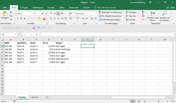
The search criterion should always be to the left of the output value.
Now let's build a search box , something like this:
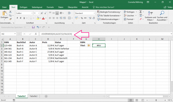
We leave the cell behind " ISBN: " blank. Next we write the following VLOOKUP formula in the cell below, here for the title (in cell H2 ):
=SVERWEIS(H1;A2:E7;2;FALSCH)
- The search criterion is in field H1 .
- It should be searched for in lines A2: E7 . The colon at A2: E7 means "to" - from line A2 to line E7.
- The output attribute is in the second column of this table - so the 2 .
- You should not only search for the input value approximately, but exactly - therefore FALSE .
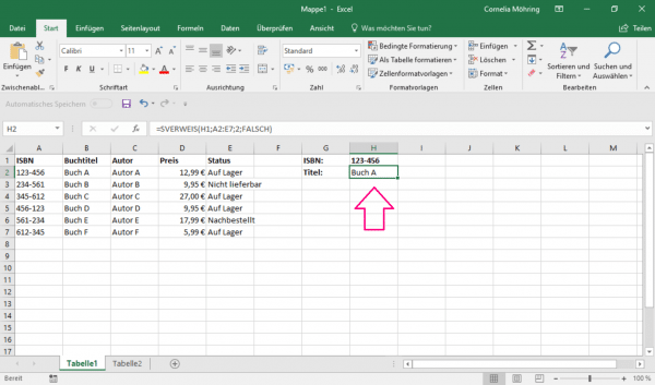
Attention: An error message is displayed here: #NV. This means that the command entered does not yet have a search term . The reason for the error is that field H1 is still empty. More explanations of VLOOKUP error messages can be found here. If you entered an ISBN there, it looks like this:
In the bookseller's example, a few more lines could be added to the search field . A VLOOKUP is now entered in each of the output fields so that the correct attribute is output. In this way, the bookseller could find out all the necessary data about the book by entering the ISBN ..
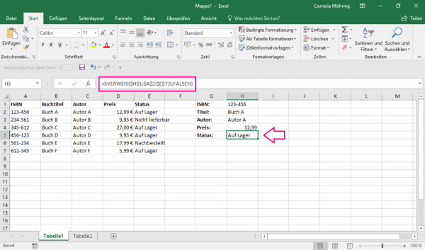
To make it easier, we've changed the formula . The values are fixed by the dollar signs . So if you now copy the formula and paste it elsewhere, table A2: E7 will still be used, and cell H1 will continue to be used as an input field . Normally, the input cells would also change when the formula was moved. If you type this formula directly into the H2 box , you can drag the box down using the square in the lower right corner . This will copy the formula into the cells below . Then all you need is
to change the specified column , so here from column " 2 " to the relevant column.
The search and output window is now complete . You can of course adapt the VLOOKUP to any search list. Unfortunately, it is not possible to search for multiple values in an Excel VLOOKUP at the same time.
The VLOOKUP in examples
So that the whole thing doesn't just stick to "dry" theory, we have now put together two more examples for you. The above example referred to looking for values in a very simple table. The following examples get a little trickier..
Creating VLOOKUP in Excel with 2 Tables
To make a search with a VLOOKUP, you can also merge data from several tables. We'll show you how to relate a VLOOKUP to two tables below.
To do this, you have to format an area of your Excel sheet as a table as described above. Repeat this for the second area as well, so that you now have two table areas in your Excel sheet. The VLOOKUP now used aims to take a search term from the first table and assign a result from Table 2. For example, table 1 can contain the personal details of a customer and table 2 the invoice amount.
Assuming that the customer names are in column A of the first table and column C of the second table, and that the billing information is in column D of the second table, one possible formula could be:
=SVERWEIS(A2;Tabelle2!C1:D10;2;FALSCH)
With this formula, the name in the first table in cell A2 is now used as a search criterion. This criterion is searched for in table 2, which goes from cells C1 to D10. The column index is set to two, and only exact results are to be output.
VLOOKUP Vacation - How to Use a Calendar
You can also do less math with a VLOOKUP. For example, you can create a calendar in Excel in which you list the holidays. Create the calendar using a template and format it as a table. As a VLOOKUP search, you can then, for example, display what is in the calendar on the respective date. These can be your own appointments or vacation appointments.
Problems with the VLOOKUP?
You might encounter some problem setting up a VLOOKUP. That is why we have put together some error messages and application errors together with the solution for you:
# NV display
As described above, sometimes only "#NV" is displayed instead of a value in the output field. This happens when you refer to a cell in the formula entered that has no or no suitable content. Alternatively, the formula can also refer to a non-existent value or a missing variable. The best thing to do is to step through your entered formula to find the loose end.
Table sorted incorrectly
For a VLOOKUP to work correctly, the search term column must always be on the far left. If this is not the case, incorrect results or error messages may occur.
#REF! Error
This error can occur if you specify a column number in the column index that does not appear in the table you have formatted. This can be the case, for example, if the specified column number is too large.
FALSE / TRUE interchanged
If you receive results that you probably would not have expected, it is possible that your entry in [Range_Reference] is incorrect. Remember: FALSE for the exact result, TRUE to find a result that is as similar as possible.