A pivot table is a special type of Excel table. Existing data can be evaluated here without changing the original table. This results in a summarized form that only contains the most important information.
Advantages of a pivot table
Above all, a pivot table facilitates clarity, as only the required data is displayed in a compressed form. The original table could have several thousand rows, but most of it contains unimportant information. Your pivot table, on the other hand, only has a handful of rows and columns, but only contains the values that you actually need.
You can read even more about pivot tables in Excel here..
Create pivot table in Excel
In the following, we will explain the individual steps for creating a pivot table using an example: In a company, the sales of various employees are to be evaluated. There are also Mr. A, B, D and F, as well as Ms. C and E. They served customers 1-7. The table shows the seller, sales and the respective branch.
The goal is to create a pivot table . It should be listed which seller made how much turnover. As a detail, it can be included how much sales were made by which customer. In this example, the specified branch is no longer required as information . It is no longer displayed in the pivot table..
Follow our step-by-step instructions or take a look at the brief instructions .
1st step:
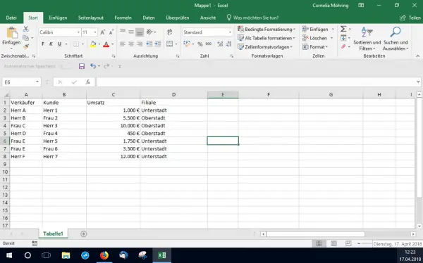 First you need to enter your values in Excel . Give each column in your table a meaningful heading .
 2nd step:
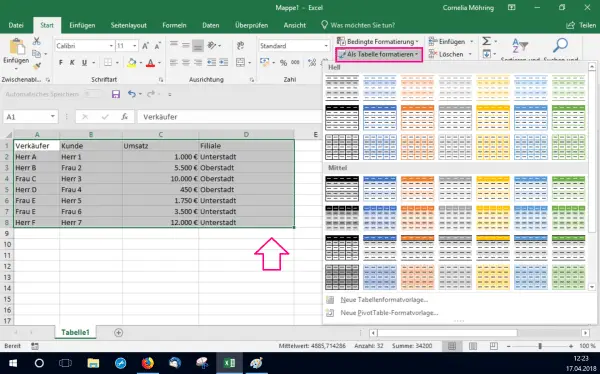 Mark then your table. Open the " Start " tab . Click Format As Table . Now you need to choose a design for your table. For clarity, we recommend a simple design in black or gray.
 3rd step:
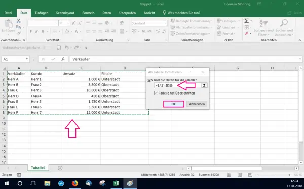 A new window is opening up. When you have marked your table (as described in the previous step), all you have to do is click " OK ". If you have already defined headings for the columns (as described in step 1), keep the checkmark next to " Table has headings ". This is extremely useful for creating the pivot table later.
 4th step:
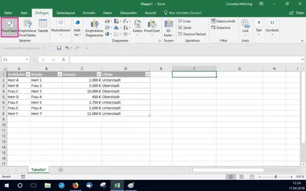 Click a field outside of your table. Then select the tab " Insert " the " PivotTable off".
 5th step:
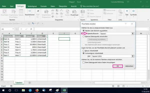 In the new window, enter your formatted table under " Table / Area: ". You have several options for this: You can mark the existing table with the mouse or enter the row or column information yourself. Alternatively, you can use the values " formatted as a table " by just entering " Table1 ". You have already formatted the values as a separate table. If you have already formatted values other than a table in the Excel file, you must adapt the number accordingly So if your values are in the second formatted table, you must enter " table2 ". Then click OK .
 6th step:
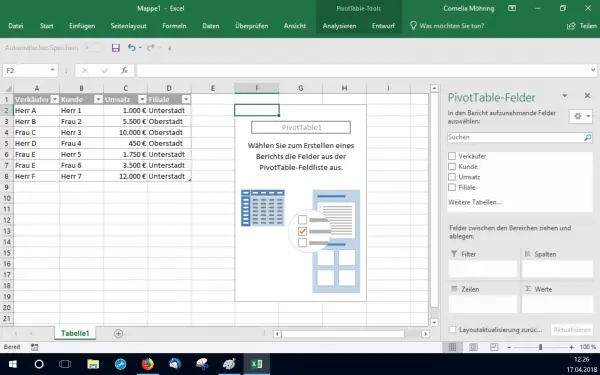 You have now created an empty pivot table . Now you need to fill it with data.
 7th step:
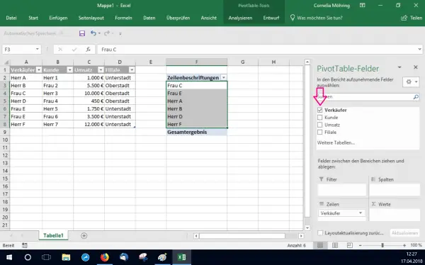 On the right side you can choose from different values. Check the box next to your base value . This is the value on which the other values depend . In the example, the base value is " seller ", because the sales generated by the sellers are to be determined. The heading " Salesperson " and the associated data have now been automatically sorted into the " Lines " section .
 8th step:
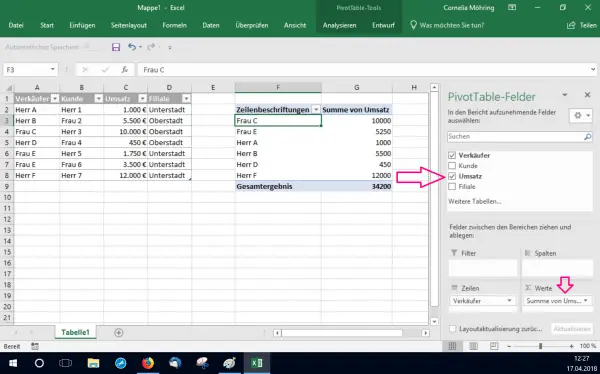 Now you have to put a tick next to the value, which depends on the base value. In this example, this is " Sales ". You can see that the heading and its content have been sorted under " Values ".
 9th step:
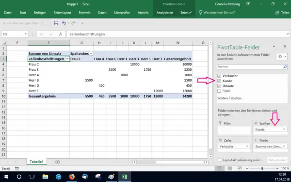 If you want, you can now set a third dependency: In the example scenario, the pivot table should also show the sales generated per salesperson by a specific customer. Therefore you have to click on the heading " Customer " and drag it into the " Columns " field. Depending on the scenario, you now have to adapt the column names of the pivot table to your requirements.
 10th step:
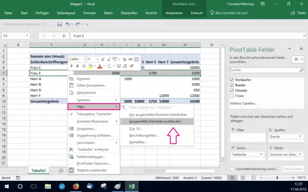 Finally, you can apply a filter . For example, a base value can be hidden . For example, if you want to display all salespeople except for Ms. E, right-click on Ms. E's cell . Select the " Filter " option in the menu . There click on " Hide selected elements ". In this way you can hide any row in the pivot table.
 quick start Guide
- Enter your values in an Excel spreadsheet . Make sure that each column has a meaningful heading .
- Now mark your table. Then click on " Format as table " in the " Start " tab and select a design .
- If you already marked your table in the previous step, all you have to do is click OK . If you have already defined headings for the columns, leave the checkmark next to " Table has headings ".
- Now select a field outside of your table . Then click on the " Insert " tab and then on " PivotTable ".
- Under " Table / range: " " Table 1 " or select your table. Then click OK .
- Put on the right side of a hook your base value to the empty to fill pivot table.
- Then check the value that depends on the base value . This value is now automatically set under " Values ".
- You can define a third dependency . To do this, the heading must be inserted in the " Columns " field .
- Now you can set a filter , for example to hide the base value. Right click on the parameter to be hidden. Then click on " Filters " and then on " Hide Selected Items ".