Google Spreadsheets (Google Sheets) are a complete tool to manage data in a comprehensive way, but at the same time simple with precise results, one of the many options that Google offers us is the ability to add reference to some sections of the data by modifying the name of the columns or rows through the name ranges..
These name ranges give us the ability to customize the work on the sheets since we can add a custom name to a group of cells, it applies to both columns and entire rows. This option does not overwrite the original cell references such as A1, A2, B1, only that it allows us to work more easily by knowing what type of data exists in a range.
Let's see how to assign a name range to a row or column in Google Sheets..
To stay up to date, remember to subscribe to our YouTube channel! SUBSCRIBE
How to pin a cell or column in Google Sheets
Step 1
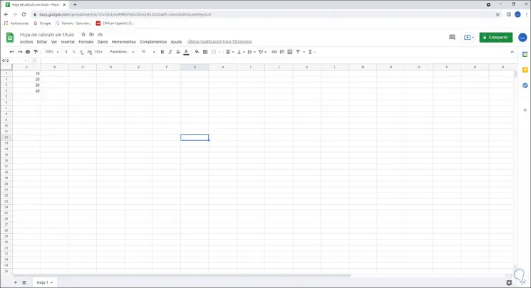
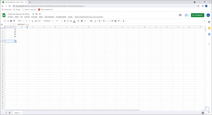
One of the first options and perhaps the simplest is to use the name box, for this we open a Google spreadsheet and we will see the following:
Step 2
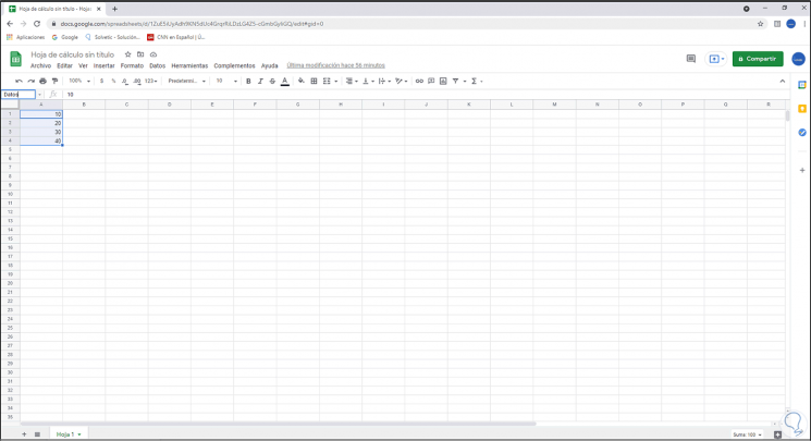
There we select the range of cells, click on the name field and enter the desired name:
Step 3
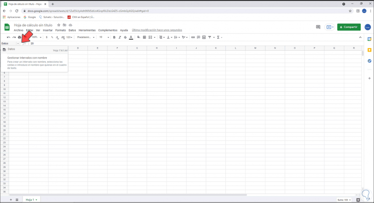
We press Enter to confirm, from the drop-down arrow we will see the name and range created there:
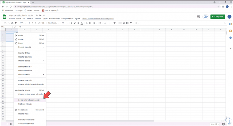
Step 4
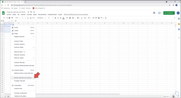
Alternatively, it is possible to select the desired range, right click on it and select "Define named interval" in the displayed list:
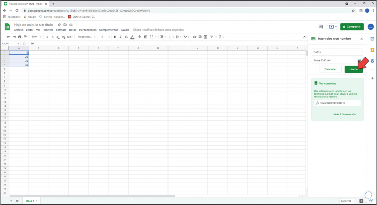
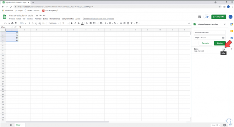
Step 5
This will open the following window, we assign the name and we can modify the range if it is the case:
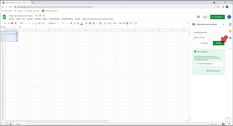
Step 6
When assigning the name we click on "Done" to confirm the change:
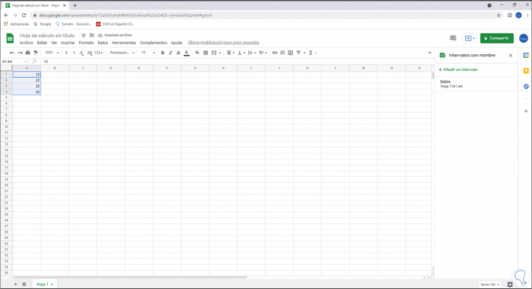
Step 7
By clicking Done the range will appear in the window and the cells in that range will be highlighted:
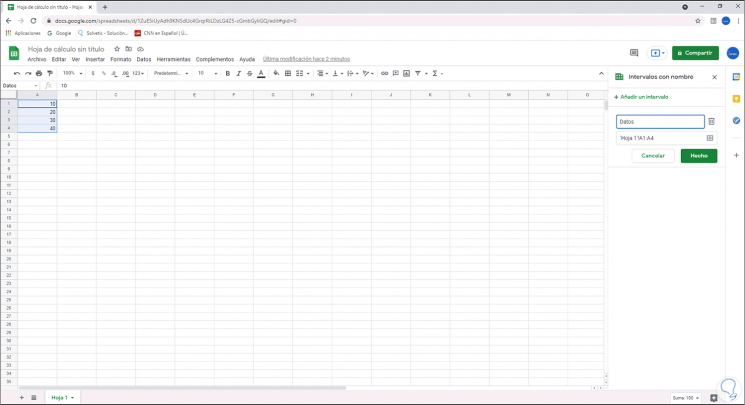
Step 8
To edit the range, we right click on any of the cells and select the option "Define named interval":
Step 9
Click on the name of the range and click on "Edit":
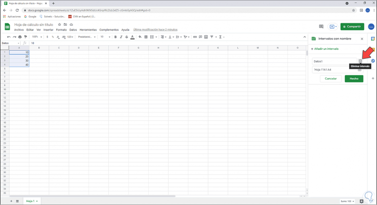
Step 10
It is possible to change the data or delete the range if it is the case:
Step 11
To delete that range we click on the trash icon:
Step 12
It is possible to use the range with any of the functions of the Google Sheets spreadsheet, for this we enter the formula and then the first letters of the name of the range:
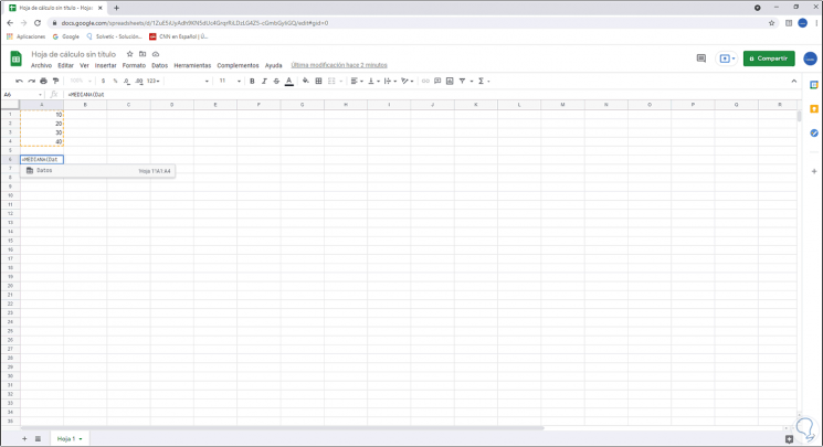
Step 13
We click on the name of the range and pressing Enter will apply the desired formula:
This is the way we can use the name ranges in Google Sheets to manage the data registered in the cells in a much simpler way, remember that it is vital to know with certainty where each of these data belongs so as not to make mistakes that affect the operation.